Early Exit Networks for Computer Vision Pt.1

Graphical depiction of a generic early-exit in neural network architectures. taken from [6]

Context

Between October 24' and February 25', I worked did my masters thesis work on a relatively new type of neural networks architecture called Early-exit neural networks. A relatively new design approach to designing neural networks that aims to reduce latency of large models. Specifically I worked with networks for computer vision (CV)

The work aimed to achieve two main goals:

Enabling an early-exit model to be production-ready

Explore the understanding on their increased performance.

The results from this small research journey were very interesting and promising, but not deep enough to produce a paper (although the work continues and we will look into publishing).

This 2-part article comes wanting to share outside my academia circle this results. The first part introduces the early-exit idea and goes into some detail on one of the SOTA early-exit models, the Local-Global ViT and explains why even though its results are promising, using it in real life environments is not so straightforward. In the second part, I'll share the work I did to make the model deployment ready and I'll go in detail on the performance studies I carried on it and the implications of this findings in future use these fascinating new models.

Important note: At the time my thesis (Oct.24 - Feb.25) the Visual-Transformer (ViT) like models were at the top of the leader-boards for many if not all the CV challenges like object detection and Image Segmentation. Naturally the early-exits research looked into ViTs. At the time of starting my thesis there was a clear trend of increasing work in this junction. Hence, we will focus solely on models based on the ViT. This even though early-exits have a history in CV way before the advent of the transformer. As we will later see, this is quite convenient since the transformer architecture is quite modular and allows for early-exits to be placed more easily.

I hope you find this novel approach as interesting as I did and perhaps useful, if you are doing something similar :-)

Introduction

AI+CV in Robotics

Computer vision deep learning models achieve state-of-the-art performance across image recognition, segmentation, and object detection tasks, making them highly attractive for robotic applications. However, these models come with a significant drawback: computational latency. The high prediction time—how long it takes a model to process an image— makes using this models in robotics not trivial, as this systems typically run on resource-constrained hardware. While computational hardware continues to improve, AI models are growing even faster in size and complexity, creating an ever-widening gap between model requirements and available resources.

Scale issue of the Transformer

I will not dive deep on the details behind the transformer or the visual transformer, for that I’ve put some excellent resources at the end of the article. You don’t need to be extremely familiar with their architecture to understand this article, but for this section it would for sure help.

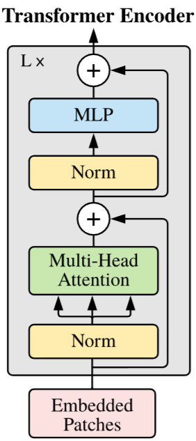
Let’s start at the base. An essential part of the transformer’s architecture is the Encoder. The encoder is essentially a chain of so-called attention blocks. They are named thus because at the hart of each block lies the (scaled dot-product self-) attention algorithm, defined as follows:

\text{Attention}(Q,K,V)=\text{softmax}(\frac{Q \cdot K^t}{\sqrt{d_k}})V

Where $Q, K, V$ are matrices computed as $Q=XW_Q$ , $K=XW_K$ and $V=XW_V$ , with $X$ being the input (Claude.ai suggested I give some explanation on what these matrices mean, but this falls outside of the scope of this article, and there are some great resources offering some interpretation on this matrices, see at the bottom)

This marvelous equation comes at a cost; The computational complexity of the entire self-attention calculation is $O(n^2)$ . I recommend referring to this great paper on the computational complexity of self-attention for details.

This present a difficult challenge: If we wanted to increase the image size by a factor of 2, to get more details and perhaps be better at prediction, we would need 4 times more computations. Even if running this calculation in GPU, the latency might increase significantly, particularly if there are many blocks with now an increased computations count.

The problem (or opportunity) of over-thinking

Increase in network size has grown directly in correlation to performance, and while there might be some over-dimension, the bigger is better mantra seems to hold so far.

One could ask, if models perform better when increasing in size, what is the limit?

Ideally, the design of a network goes over some iteration on its hyper-parameters, one being the amount of neurons added to the network, and the size chosen should be close to the best performing one. If when designing a model, increasing its size brings performance down, it means that the model’s additional neurons were detrimental for the overall performance of the model, and a smaller model is the best performing. In other words, within the scope of the network’s size, the optimal architecture for a dataset is that one with the highest accuracy. But that does not mean is the optimal for ALL data in the dataset.

This phenomenon of additional processing is called over-thinking, “which occurs when a DNN can reach correct predictions before its final layer” [5].

This phenomenon occurs because neural networks are typically designed to handle the most challenging examples in a dataset. However, not all inputs require the full computational depth of the network. Consider image classification: a clear, well-lit photo of a cat might be correctly identified after just a few layers of processing, while a blurry, partially occluded image of the same cat might require the full network depth. The "overthinking" problem emerges when we force simple examples through unnecessary computational layers, wasting resources without improving accuracy. In essence, the optimal network depth varies per input, but traditional architectures use a fixed computational path regardless of input complexity.

Considering this over-thinking problem, what if there was a way to avoid unnecessary runs through attention blocks? What if we could use just the right amount of attention blocks and prevent using the rest, thus saving latency time?

Enter early-exits…

Early-Exits

Early-exit design is an approach to make larger models act faster and still preserve or even improve they performance.

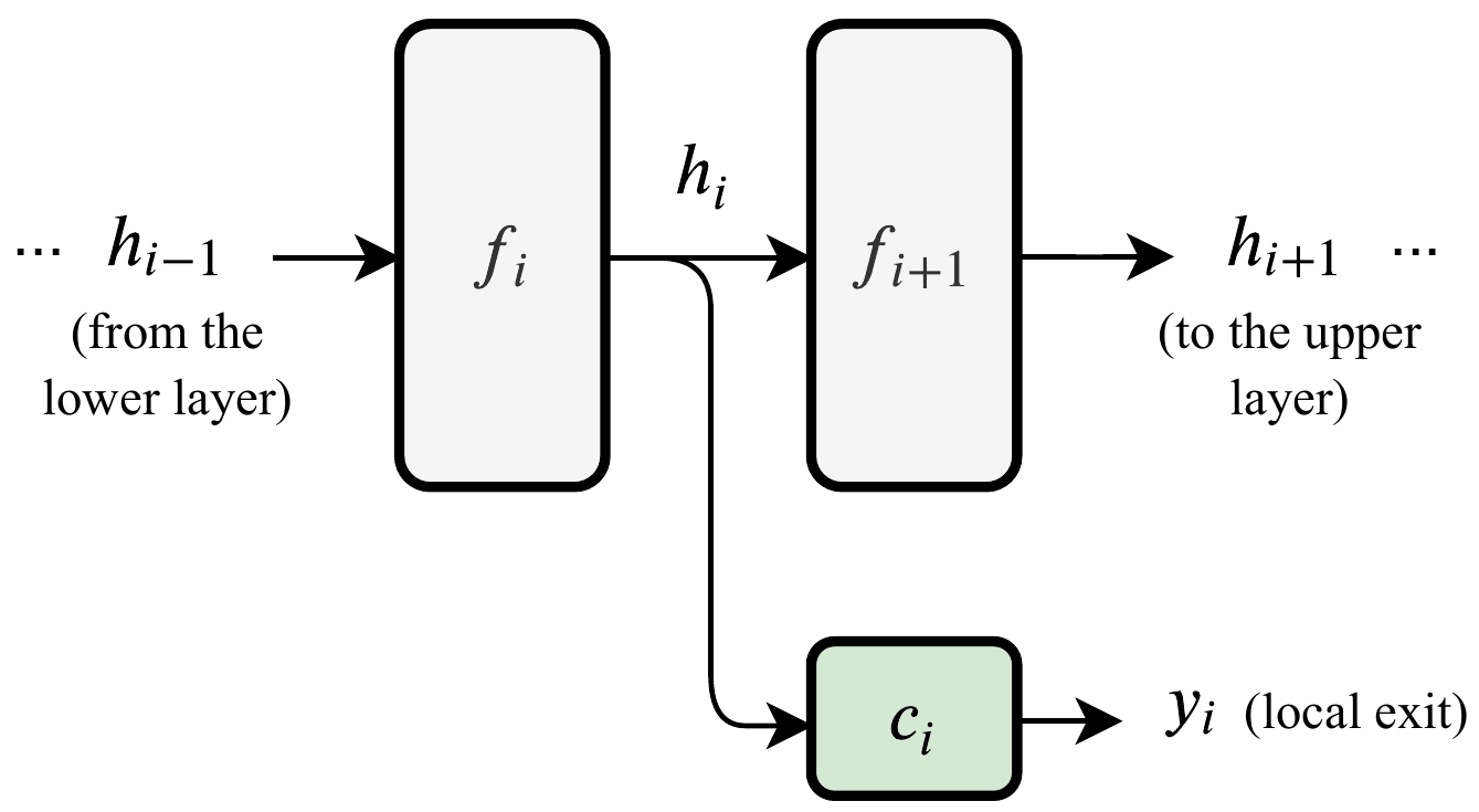
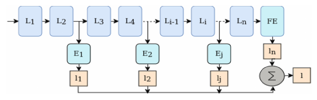
As mentioned before, in a typical neural network, latency is fixed, and it stays fixed no matter the characteristics of the given data. The idea is then to attach additional computational flows to the model’s ‘static’ one, with the intention of producing outputs faster than by just using the static network. Then, discriminating with some heuristic, such early output is potentially taken as the model’s output.

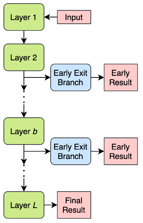
Schematic representation of early-exits in a neural network model [3]

The figure above shows the general idea behind early-exits. If any of the early results passes the determined heuristic, the computation stops and the prediction is yielded.

Typically the longest computational path is called the backbone. In models that are extended with early-exits, this would be the the un-extended graph. The early-exits are sometime called branches.

Early-exit design

Designing early-exits for a network is essentially answering 4 questions:

Architecture: What kind of branches to attach?

Placement: Where to attach these branches?

Training: How to train this branches?

Exit policy: Through which branch to exit?

There has been a considerable amount of work done on answering this questions and covering all considerations fall outside of the scope of this article. I want to give an overview on how this challenges have been approached, and and the end of the section will mention the references that provide excellent in-detail explanations.

Architecture and Placement

The design of early exit branches depends critically on their placement within the network. Since branches receive only partially processed information, their architecture must compensate for this limitation while minimizing additional computational overhead.

For Vision Transformer backbones, research has consistently shown that CNN-based branches perform better in shallow layers, where they can capture local features that transformers initially struggle with. Conversely, attention-based branches excel in deeper positions, where the transformer has already captured sufficient global context.

This insight led to hybrid approaches where different branch types are strategically placed: convolutional branches early in the network for local feature extraction, and attention-based branches later for semantic understanding. The key finding is that early-exit models benefit most from heterogeneous branch architectures tailored to their specific positions rather than using identical branches throughout.

A good example of this process is the work of Multi-Exit Vision Transformer for Dynamic Inference [3]. They attached 7 different branch architectures to a ViT backbone and compared each locations accuracy of all branch options, bench-marking their performance in the CIFAR10 and CIFAR100 datasets.

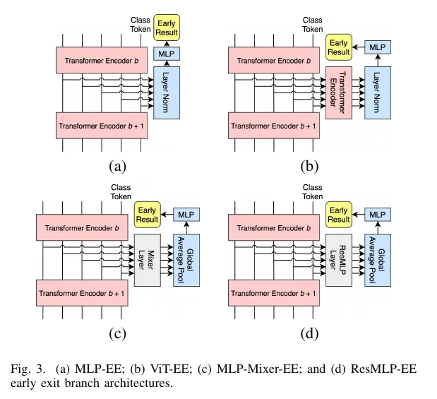
From their results we can see that in early locations, CNN branches out-perform ViT based ones in early positions, likely due to the combination of convolution with early attention states. Conversely, at later staged ViT-like branches take the lead, perhaps since the many attention blocks used at that point capture enough information before being processed for exiting.

A very noteworthy conclusion form these work, is that an early-exit model can have branches with different architectures, each one selected to perform best at their location.

Training

Training early-exit models requires careful consideration of how to optimize multiple prediction heads simultaneously. Three main approaches have emerged:

Joint training optimizes all branches and the backbone simultaneously through a single loss function that combines predictions from all exits. This approach ensures consistency across the network but can be computationally expensive.

Layer-wise training focuses on training each exit with its associated backbone layers, either including all preceding layers (separate training) or only the layers that directly contribute to that specific branch (branch-wise training).

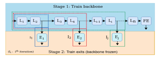
Two-stage training first trains the backbone to completion, then freezes its parameters and trains only the exit branches using techniques like knowledge distillation from the final layer.

The choice depends on computational resources, implementation complexity, and desired flexibility. Two-stage training often provides a good balance of performance and simplicity for practitioners.

Visual representation of the ‘joint’ training strategy [4]

Visual representation of the ‘*two-stage’* training strategy [4].

There are more complex strategies, like knowledge-distillation or the so-called hybrid strategies, but they are for the most part combinations of these ones mentioned here.

Choosing a strategy depends on a number of factors. The work in [4] score these strategies with 5 indicators: Computational complexity, Implementation complexity, Inter-branch training coordination, flexibility and transfer learning potential. For a deeper understanding of the options out there and their implication I highly recommend reading their work.

Exit strategy

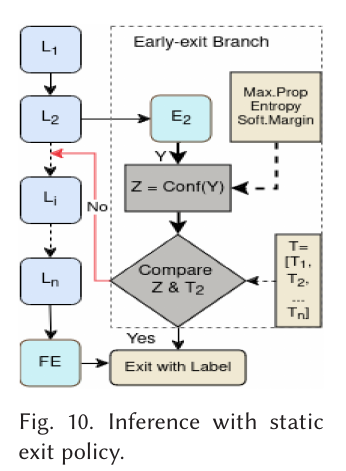
Exit strategy or exit policy, refers to the decision mechanism to determine when and which exit’s prediction to use. Its common for this policies to be rule-based or static. The two most common are Max-SoftMax and Entropy.

The Max-softmax strategy compares the confidence of an early-exit’s prediction to a threshold value, and for the Entropy strategy, predictions are considered confident if the entropy of the prediction vector falls below a determined threshold.

There are other strategy types. Its also common to find learned policies or policies of inclusion, those where the intermediary exits are not taken as output but as a alternative processing to aid in the final prediction— but these fall outside of this scope.

The LGVIT model

Meet LGVIT

In 2023, Xu et al. [2] presented LGViT, an early-exit model with very promising results, as they showed significant computation savings with little compromise in accuracy. Their work involved taking many of the useful insights from past research in term of branch architecture and training and putting it all together.

They carried themselves a branch type study and came to two conclusions:

Convolution-based exits can offer good feature representation in shallow layers of the ViT

Attention-based exits extract target semantic features if places late enough in the model.

Very similar to the insights from the authors of Multi-exit vision transformer!

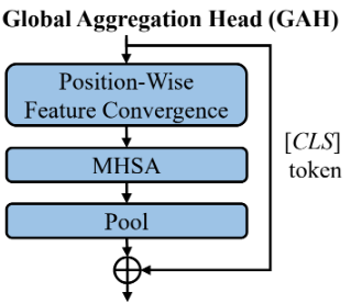
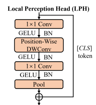
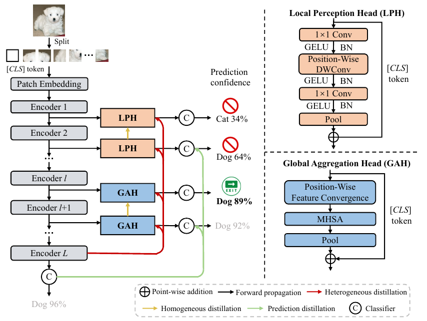
Based on this, the LGViT authors designed two types of branches, which they called Local Perception Head and Global Aggregation Head. The first one has convolution at its core, with some of the kernels being dependent on the position of the head. The second one aggregates by means of pooling adjacent features and then applies dot-product attention to the pooled features. Here two the pooling window size is position dependent.

As Exit strategy, the authors resorted to the well used max-Softmax strategy we mentioned earlier. Formally, the strategy compares the highest class probability $c_m(p^m)$ in the $m$ exit’s prediction distribution to a determined threshold $\tau$

$\text{For exit $m$}$ :

$c_m(p^m) \gets \max_C (p^m)$

$\text{if }(c_m > \tau)$

$\textbf{Exit}$

The threshold value can be different for different exits, but its common for it to be a fixed value. In the case of LGViT, the authors’ published value was 0.8. This decision should not be overlooked. As we will see later on, this can have major implications in the performance increase.

For training, the authors implements a two-stage custom training scheme. First, an end-to-end approach helps the backbone ViT achieve high accuracy. In the second stage, the parameters of the backbone are frozen, and only the exiting heads are updated through self-distillation techniques. This procedure helped minimize information loss between the heterogeneous exit architectures and facilitated knowledge transfer from deeper to shallower exits.

Results

The researchers evaluated LGViT across multiple Vision Transformer architectures, including ViT, DeiT, and SWIN models.

The following table shows a segment of the results from LGViT and its comparison to the baseline model ViT-B/16 (One of the original ViT iterations; Base model with 16x16 image patches)

Method	# Parameters	CIFAR100	FOOD101	ImageNet-1K
ViT-B/16	86 M	90.8% \| 1.00 X	89.6% \| 1.00 X	81.8% \| 1.00 X
LGViT	101 M	88.5 % \| 1.87 X	88.6% \| 2.36 X	80.3 \| 2.7 X

Take a look at the implications. In all three cases, the model gains significant speed ups —between 87 and 170 % — at a cost of ~2% in accuracy.

Slicing the computations —and thus reducing latency as well — in more than half sure at little accuracy cost sure feels like something useful for time restricted tasks.

Implementation

The LGViT implementation maintains a structure similar to the original Vision Transformer (ViT) model (ViT-B/16), retaining the same embedding, transformer block, and final MLP head components. The figure hereunder shows the class diagram of the model’s implementation.

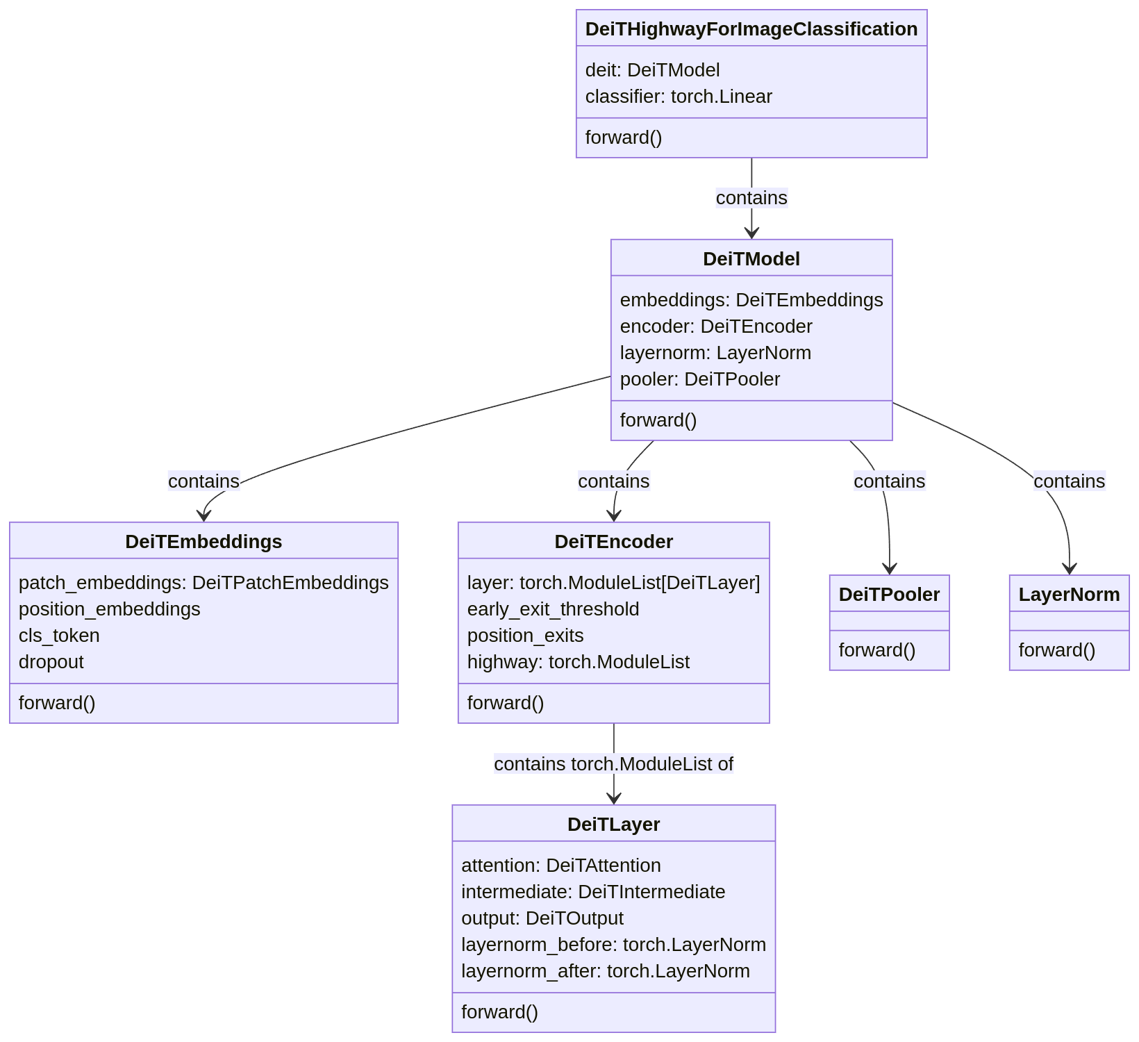
The implementation unifies both ViT and DeiT models under a single structure, with naming conventions primarily reflecting DeiT terminology. This unified approach enabled the authors to experiment with different backbone architectures more efficiently. The forward pass through the model follows a specific flow pattern, presented in the following block diagrams.

The first figure shows the high-level flow through the entire model, while the second illustrates the encoder's operation with early-exit mechanisms.

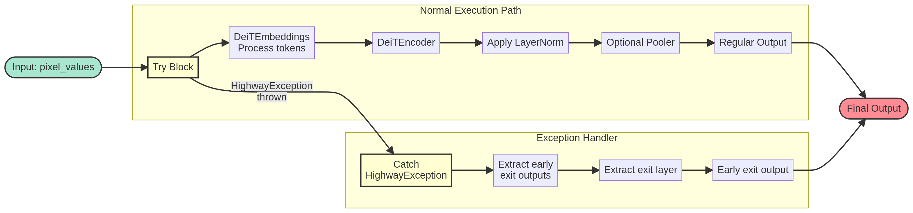
The implementation utilizes try/catch statements as the exit mechanism. When exit conditions were met, the determined DeiTLayer throws a HighwayException, which is then caught by the DeiTEncoder.

Challenges beyond design

Early-exit models in production(?)

Despite their potential, adoption of early-exit models in production environments
is challenging due to the dynamic nature of their computational graph. At code level, the mechanisms that change the flow of the computation are known as control-flow statements.

Because they are very common for all types of computations, it might even sound a little ridiculous to say that they require special attention when implementing them for neural networks that are to be used in production systems. Why is that? It all comes down to traceability. More specifically, to exportability.

Production environments, especially in edge computing scenarios, in order to maintain

Furthermore, such environments benefit from remaining agnostic to the development frameworks used to build the models they employ. so that replacement of older models with newer, better performing ones is seamless. The ONNX (Open Neural Network eXchange) standard addresses this need by providing a framework independent representation for neural networks.

💡

You can read more on ONNX in these two resources:

Understanding ONNX

ONNX explained

While neural networks are typically built using powerful frameworks like PyTorch or TensorFlow that come with a cornucopia of development tools, these same frameworks represent undesirable dependencies in production. Converting models created with any framework to ONNX format simplifies their adoption in framework agnostic production environments.

This context highlights the adoption challenges for early-exit models: until recently, capturing their dynamic nature in ONNX was very cumbersome, when it was not impossible. For PyTorch, for instance, the API for tracking and exporting flow control operations was only added in their 2.6 version earlier this year. The torch.cond operation allows for graph computations of the model to be traced. This allows for the model to have dynamic behavior, “simply” by replacing the traditional if:... else: syntax with the new torch.cond(pred, true_fn, false_fn, operands).

Bottom line, what’s important to take away from this short section is the following:

In order to use Models developed in heavy frameworks in production environment without having to install such frameworks, the models need to be exported into a format allows their decoupled use. The ONNX standard is the most prominent option for this.

early-exits models have a dynamic computation. That is, the computation path they follow among the many possibilities inside the model might change from input to input.
1. Until recently, exporting them into ONNX was not possible
1. Now, while possible, the implementation needs to be implemented in a way to do so. For example, in PyTorch, using the special operation torch.cond

Conclusion

In this 1st part, we’ve learned the basics of early-exit neural networks as well as some of their advantages and challenges. The following takeaways are most key:

early-exits promise to reduce the latency of big slow models to make them very attractive for environments that could benefit from them.

Research focused on ViTs with early-exits shows that a combination of branch architectures helps most. LGViT is one of the latest most promising results.

Beyond their design, some care is needed when implementing this networks, so that they can be deployed to the environments that could benefit from them the most.

In the next part, I’ll delve on the modifications I did to the LGViT model to make it production ready. Additionally, I’ll share the results of the performance study I conducted on this model by bench-marking it against the CIFAR100 dataset. We will see how the performance is impacted by implementation as well as by the characteristics of the dataset.

Hope to see you there!

Acknowledgements

I would like to thank my professor advisor, Lazaros Nalpantidis as well as my co-advisor, PhD-candidate Fabio Montello, both from the Perception and Cognition for Autonomous Systems group at DTU.